There’s an awful lot of excitement around artificial intelligence and machine learning, and how they’re going to devise solutions to problems that will change the world in ways we can only dream of today.
Every week there is news of a breakthrough that allows some AI to beat the best humans at games, understand chemical interactions, or drive a car by itself. But what exactly does it mean for a machine to learn, and how does it do it?
Well, I’ve done my best to explain those ideas as simply and intuitively as I can. I’ve tried to avoid as much mathematics as I can because I find that it can often get in the way of an intuitive understanding for most people, and there is no shortage of comprehensive mathematical introductions to the subject for those who want it.1
I. Problem solving
Let’s start with a simple exercise. For anyone who has some idea of programming, this should be simple. How might we write a computer program that can tell if a number is odd or even?
if number divided by two has a remainder:

    number is odd

otherwise:

    number is even
This is simple enough. We have a mathematical solution to the problem and it isn’t difficult to convert this into code that a computer can understand. Fundamentally, this is all we are ever doing when we write code. Find a way that the problem can be solved, and encode that process as instructions written in a way that can be understood by the machine.
But what happens if we can’t solve the problem, or if we solve it so easily that we can’t explain how?
Take a look at this picture, we easily recognise which one is the cat, but if I ask you how you know which is which could you give me a good explanation? They both have four legs, are covered in fur, and have pointed snouts. It’s not so easy to come up with some unique set of measurable features that differentiate between a cat and a dog. So how could we ever expect to program a computer to identify which is which if we can’t tell how we do it ourselves?

There seems to be something happening in our brains that allows us to identify what we’re looking at without consciously thinking about it. We don’t think about what makes a cat different from a dog, we learn to identify them after our parents teach us when we see them as children.
So how exactly do we encode instructions into the computer if we don’t even know how we solve the problem? What we need is to be able to show a computer what a cat is and have it work out for itself what features distinguish a cat from a dog.
Learning from data
Instead of having to expressly encode our solution for the machine, we need to be able to teach the machine how to figure out the solution for itself.
This is what we mean by machine learning, we don’t teach the machine how to solve the problem. We simply give it the problem, ask it to make a guess at the answer and correct its mistakes. If we do this repeatedly we should see improvement in the performance as it starts to build on guesses that were right and discard ones that weren’t.
Often we may require vast amounts of data because although we humans can learn from a very small set of data, even our best learning algorithms aren’t quite there just yet.
This simple process should in theory eventually result in something that we can now use to solve our problem.
II. Making predictions
One of the simplest ways of following this process is through linear regression. Fitting a line to data. You probably learned this in school as finding the line of best fit, the line that most closely fits all of the data.
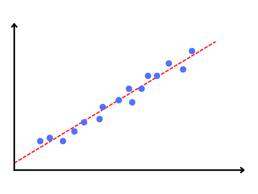
Our intention is that by finding a line that fits our data most closely, we can then use a value on one axis to predict the value of the other. Simply put, we want to use data to make a prediction.
A practical example of this might be if we measure how many ice creams are sold from our ice cream parlour each day of the year, along with the corresponding temperature that day. We would expect to sell more ice cream on hot days, and if we plot a simple linear regression model we should be able to use the temperature forecast to predict how many ice creams we will sell on any given day.
Optimising our regression line
When we do this manually it is a simple process. Slide the line around the graph until you find a place where it looks closest to the most data points. Eyeballing the process is not the best practice, but it does give us a nice intuition for what we’re doing.
If we really care about the right answer though, we probably want to be more precise than this. So now we need to break out some numbers and start calculating; if we work out just how close we are to each data point, we can then evaluate our overall performance as the sum of the distances from each data point to the line. The greater the total distance, the further we are from all of the data points in aggregate.
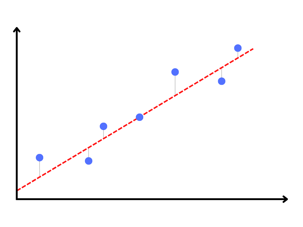
Now that we have a metric to tell us our performance, we can use it to make changes to the placement of our regression line, until we are able to find the placement with the minimum total distance across all data points.2
So to recap, we have some data and we are trying to find a line that best approximates it, so we can use it for making predictions. We have a way to evaluate how closely our prediction line represents the data, and we can use that information to improve it.
Making our best guess and then improving it based on how well we did. That is starting to sound like learning to me.
III. Neural Networks
Theoretically speaking, a neural network is just a mathematical function that is flexible enough to solve any problem.
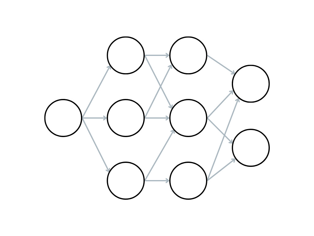
A neural network is a collection of artificial neurons which are connected together in layers, roughly based on the way a human brain works. Much like the human brain we can feed data into the neural network, and see pathways of neurons activate as data passes through the network, eventually spitting out a result for us.
But what does it mean for a neuron to activate and how does it work?
Neurons
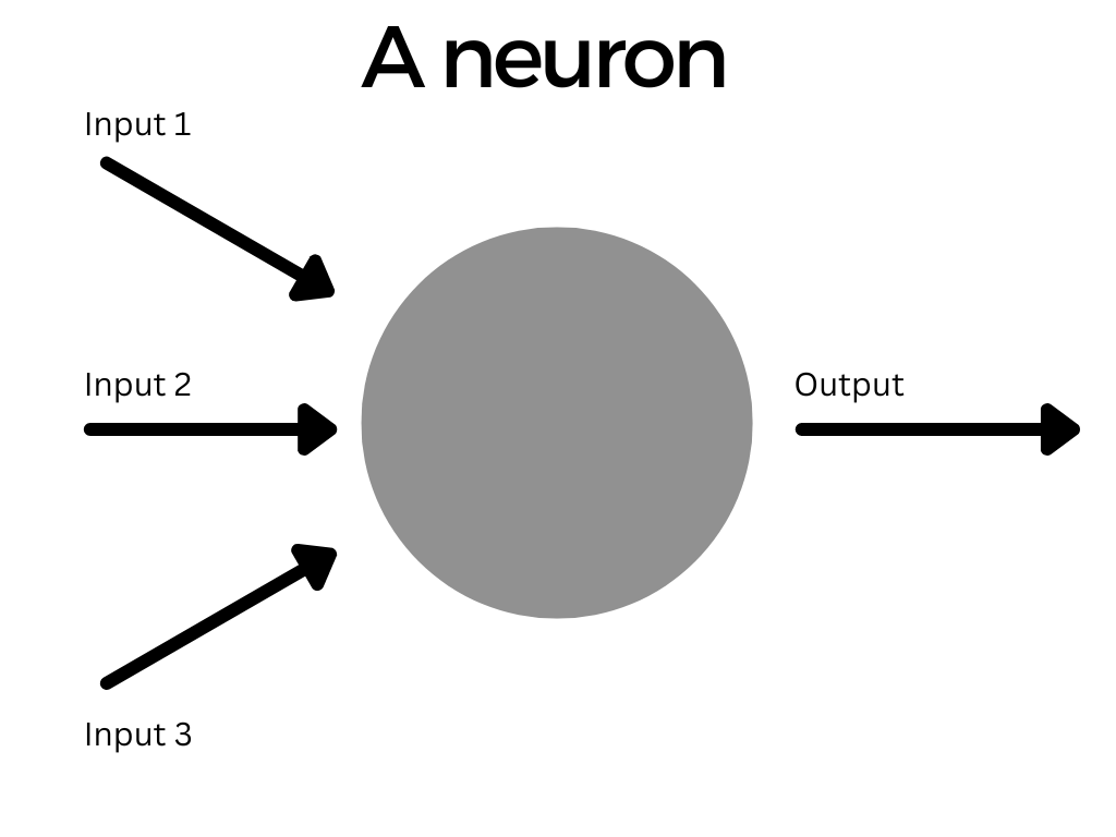
The most basic piece of a neural network is a neuron, without them we would have no network.
We can think of each neuron as a little box which takes in some numbers as input, does something to them, and spits out a single number as the output. The output from one layer then becomes the input for the next, and so on. This output is what we mean when we talk of the activation of a neuron.
Weights and Biases
A neuron can take in multiple inputs, either from the input data itself if the neuron is in the first layer, or from multiple other neuron outputs in a previous layer.
The output of a neuron is the weighted sum of all its inputs, plus a bias term, that we then pass through something called the activation function. This can be expressed mathematically like this:3

Let’s try to understand this more intuitively; we want to take each input that the neuron receives and determine how important it is to make our neuron activate. We do this by multiplying the input by a weight.
A weight in a neural network is a parameter that we can tweak to determine how much a neuron activates. Each connection between neurons has its own weight. As we train the network, the weights for every connection are changing to find the optimal levels for activating neurons in some situations but not others.
If we think about our cat or dog example, imagine the input to a neuron is a group of pixels that represent a pointy ear, we know that this is more important for recognising a dog than a group of pixels representing some grass. So in this case the weight should be higher for the ear pixels and lower for the grass pixels.
So we have a neuron that will activate more strongly when the input it receives is pixels representing an ear than ones representing grass; we can think of this as sort of like an ear detector. Bear in mind that we are not programming the neuron to look for ears or grass in an image, this is simply an example of how a neuron might respond to patterns in the data.
After we have multiplied each input by a weight, we then add them all together to get a weighted sum of our inputs which represents how much the neuron should activate. If we look back at our equation, we can see this is the main part of it.

Next, we have the bias term. This is an extra number that we add to our weighted sum, and it serves as a threshold of sorts.
If we want the neuron to activate very easily then we might add a high bias, as this will increase the overall value of the neuron. If we don’t then we might have a very small bias so the activation depends more on the weighted sum of inputs.

In any case, we’ve taken our weighted sum of inputs and added a bias term. The final step is to pass this value through an activation function.
It is also worth noting at this stage, that when we first start we don’t know what a good weight or bias is for our neurons so we just pick a random number (no, seriously) and then update it during training.
Activation Functions
This is where the magic happens. Activation functions introduce nonlinearity into our network, allowing us to make nonlinear predictions from our data. This is just a fancy mathematical way of saying they let us build a model that can do more than just work with straight lines like our linear regression model earlier.
If we didn’t have activation functions then all we would have is a collection of neurons modelling linear relationships, and when we add them together, we still get a linear relationship because that’s just how maths works. That’s not very useful because in the real world things are complicated and weird, and so they usually have complicated and weird relationships.
Imagine we are trying to distinguish between a cat and a dog, but all we know is the height of the animal. In that case, we might expect to see data like this.
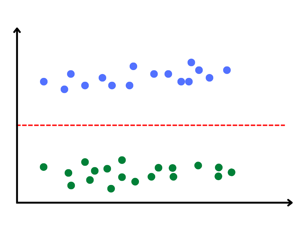
If we only have big dogs and small cats, it is very easy to use a single straight line to split the two groups. In this simple case, a linear model works. But what if we have more than just the height of the animal? If we have lots of variables like weight, length, age, pointiness of ears, size of paws, and so on we can very quickly see that there is no way we could split between dogs and cats with a simple straight line if we plotted all of those data points in a graph.
This is the reason we need nonlinearity. In the real world, most problems interesting enough to bother solving require nonlinear models.
Anyway, that’s enough maths for now I think. In short, activation functions are what make neural networks so powerful, by allowing us to combine linear layers together we can build complex nonlinear models that let us solve all sorts of interesting problems.
Back inside our neuron we take our weighted sum and bias and run it through the activation function. In this case, I’m using sigmoid which will squish the result down to between zero and one. That may be useful for some problems and others may require a different function. Don’t worry too much about that for now, I’m planning a longer post about the different types of activation functions and why we use them.
But as you can see, we’ve arrived back at our full equation from before. This is everything that goes on inside each and every neuron in our network.
Networks
Now that we understand neurons and their parameters, we can start to put them together into larger networks.
We can have a network with only a single layer, but by adding multiple layers together we can increase the complexity of the network which should allow it to learn far more than a single layer alone.
Each neuron takes input data and multiplies the values by some weight and adds a bias before passing this value back as its output. Other connected neurons take the output from previous layers and use that as their input, with the data making its way through the network until it is finally passed back out at the output layer.
Training
Now that we understand how a network goes from input to output, it’s time to talk about how we train it to give a useful output.
So far we have a network full of connected neurons arranged in layers. Our weights and biases have been randomly picked, and we’re ready to learn. If we give this network any data it will give us an output, but it won’t be any better than a total guess at first, because that is essentially all it is right now. We need to train the network to get better.
The training process is pretty straightforward:
- Feed in data to go through the network and receive an output prediction.
- Evaluate this prediction to determine how accurate it is.
- Update the weights and biases in the network to produce a more accurate prediction next time.
- Repeat until done.
Our first step is to take in data and run it through the network to make a prediction. So for example we input a picture of a cat into the network and allow it to guess whether it is a cat or a dog. We call this a forward pass; running data through the network to get a prediction.
Once we have our prediction we need to determine how accurate it is, which we can do with a loss function. There are lots of different loss functions that we can use depending on our specific situation,4 but in simple terms what we are doing is comparing the correct answer to the predicted one the model gave to see how well it did.
In our case, we want our dataset of cat and dog pictures to come with labels for which is which, and we can use this label as the “correct answer” when comparing against the prediction.
All that is left for us to do is take our loss value and use it to update our parameters. Using the magic of calculus in a process known as backpropagation, we are able to calculate a gradient for each weight and bias in the network. What this gradient does is tell us exactly what will happen to the loss value if we make changes to the parameter. We call this a backward pass.
Given that we now know precisely what changes to make for each parameter to minimise the loss, we go ahead and make little updates5 to each one to make the predictions better next time.
By repeating this process over and over we can reduce the total loss to a very low level, which tells us that our overall performance from the network is very high.
Note: There is no objective measure for ‘good’ performance from a model. Every model is different, 90% accuracy may be good enough for one model, but not for another.
The end result is we should now have a neural network that can behave like any other computational function; we give it some input data and it should return the correct answer.
IV. Summary
Ok, that was a lot to process, so here’s a short summary of everything covered.
In a normal computer program, we work out a set of instructions that will solve a problem, and then write them in a programming language for the computer to run. Machine learning problems tend to be ones that we aren’t sure how to provide the instructions to a solution, so instead, we must help the computer figure it out for itself.
We do this by giving data to the machine so that it can try to find patterns. We then train the machine to solve the problem by asking it to guess the answer, and then correcting it when it is wrong so it can improve its next guess. We do this until it seems to have reached a point where it makes accurate guesses every time.
This all sounds a little hand-wavey about how long exactly we should be training, and how we know it has worked. And in some ways it is. There’s a lot of art in the science here, there's often no single correct answer to these questions and in many cases, it is just something of an intuition that practitioners build up over time with experience creating and working with models.
As we can see there is nothing magical or wildly complicated going on inside a machine learning model. It’s just a lot of linear algebra and calculus masquerading as intelligence. Maybe one day we will build models that are truly intelligent, but for now, they’re just applied maths.6
Anyway, that’s probably enough for one post.
Footnotes
- Maybe in the future, I’ll try writing a more mathematically comprehensive introduction to some of these ideas. It would certainly be an interesting exercise to see just how well I am able to distil the maths into an easily digestible form.
- This is only using two variables for our data (represented via the x and y axes), but in reality, we would probably have far more than two dimensions. This makes it more complex to visualise but the process remains the same.
- Don’t worry if you can’t understand this, I’ve added it for completeness but it is not essential that you can read it.
- I am planning a longer exploration of loss functions in another post, but all that matters here is our intuition that a loss function is comparing prediction against a target to give us a measure of how well the model performed.
- We don’t want to make too big of a change in one go, it can accidentally change too much and cause unstable learning. But we also don’t want to make too small changes either or we’ll never finish learning. This is known as finding the ideal learning rate, and it’s as much an art as a science.
- Yes, I know that when we look closely enough at a human brain it’s just lots of simple neuron activations, and maybe true intelligence is simply an emergent property of a sufficiently complex system. But that’s an entirely different (and highly interesting) discussion.